Flip Your self right into a 3D Gaussian Splat | by Sascha Kirch | Mar, 2024

Final summer time a non-deep studying technique for novel view synthesis has entered the sport: 3D Gaussian splattig. It’s a technique to symbolize a scene in 3D and to render photographs in real-time from any viewing route. Some even say they’re changing NeRFs, the predominant technique for novel view synthesis and implicit scene illustration at the moment. I believe that’s debatable since NeRFs are rather more than picture renderers. However that’s nothing we care about at this time… Right now we solely care about crisp wanting 3D fashions and that’s the place 3D Gaussian splatting shines 🎉

On this submit we’ll very briefly look into Gaussian Splatting after which swap gears and I’ll present you how one can flip your self right into a 3D mannequin.

Bonus: On the finish I’ll present you how one can then embed your mannequin in an interactive viewer on any web site.

So, let’s go!

1. What are Gaussian Splats?
2. Let’s Flip Ourselves right into a 3D Gaussian Splatting
3. Conclusion and Additional Assets

3D Gaussian splatting is a method to symbolize a scene in 3D. It’s really one in every of some ways. For instance you might additionally symbolize a scene as a set of factors, a mesh, voxels or utilizing an implicit illustration like Neural Radiance Fields (aka. NeRFs).

The muse of 3D Gaussian Splatting has been round for fairly a while main again to 2001 to a classical strategy from laptop imaginative and prescient referred to as floor splatting.

However how does 3D Gaussian Splatting really symbolize a scene?

3D Illustration

In 3D Gaussian Splatting a scene is represented by a set of factors. Every level has sure attributes related to it to parameterize an anisotropic 3D Gaussian. If a picture is rendered, these Gaussians overlap to kind the picture. The precise parameterization takes place in the course of the optimization section that matches these parameters in such a means, that rendered photographs are as shut as doable to the unique enter photographs.

A 3D Gaussian is parameterizedwith

• its imply µ, which is the x,y,z coordinate in 3D house.
• its covariance matrix Σ, which could be interpreted because the unfold of the Gaussian in any 3D route. For the reason that Gaussian is anisotropic it may be stretched in any route.
• a shade often represented as spherical harmonics. Spherical harmonics permit the Gaussian splats to have totally different colours from totally different viewpoints which drastically improves the standard of renders. It permits rendering non-lambertian results like specularities of metallic objects.
• an opacity 𝛼 that determines how clear the Gaussian shall be.

The picture bellow reveals the affect of a 3D Gaussian Splat with respect to some extent p. Spoiler: that time p would be the one related if we render the picture.

How do you get a picture out of this illustration?

Picture Rendering

Like NeRFs, 3D Gaussian Splatting makes use of 𝛼-blending alongside a ray that’s casted from a digicam via the picture aircraft and thru the scene. This mainly signifies that via integration alongside a ray al intersecting gaussians contribute to the ultimate pixel’s shade.

The picture bellow reveals the conceptual distinction between probably the most primary NeRF (for simplicity) and gaussian splatting.

Whereas conceptually related, there’s a giant distinction within the implementation although. In Gaussian Splatting we don’t have any deep studying mannequin just like the multi-layer perceptron (MLP) in NeRFs. Therefore we don’t want to judge the implicit operate approximated by the MLP for every level (which is comparatively time consuming) however overlap varied partially clear Gaussians of various measurement and shade. We nonetheless must forged at the very least 1 ray per pixel of the picture to render the ultimate picture.

So mainly via the mixing of all that Gaussians the phantasm of an ideal picture emerges. In case you’d take away the transparency from the splats you possibly can really see the person gaussians of various measurement and orientation.

And the way is it optimized?

Optimization

The optimization is theoretically easy and simple to grasp. However after all, as at all times, the success lies within the particulars.

To optimize the Gaussian Splattings, we’d like an preliminary set of factors and pictures of the scene. The authors of the paper recommend to make use of the construction from movement (SfM) algorithm to acquire the preliminary level cloud. Throughout coaching, the scene is rendered with the estimated digicam pose and digicam intrinsic obtained from SfM. The rendered picture and the unique picture are in contrast, a loss is calculated and the parameters of every Gaussian is optimized with stochastic gradient descent (SGD).

One of many vital particulars price mentioning is the adaptive densification scheme. SGD is simply succesful to regulate the parameter of present Gaussians, however it can’t spawn new ones or destroy present ones. This would possibly result in holes within the scene or to lack of fine-grained particulars if there are too few factors and to unnecessarily giant level clouds if there are too many factors. To beat this, the adaptive densification technique splits factors with giant gradients and removes factors which have converged to low values.

Having talked about some theoretical fundamentals let’s now swap gears and leap into the sensible a part of this submit, the place I present you how one can create a 3D Gaussian splatting of your self.

Be aware: The authors recommend utilizing a GPU with at the very least 24GB however you possibly can nonetheless create your 3D Gaussian Splats utilizing some tips I’ll will point out after they should be utilized. I’ve an RTX 2060 cell with 6GB.

These are the steps we’ll cowl:

1. Set up
2. Seize a Video
3. Acquire level cloud and digicam poses
4. Run the Gaussian Splatting Algo
5. Publish processing
6. (Bonus) Embed your mannequin on an internet site in an interactive viewer

Set up

For the set up you possibly can both leap over to the official 3D Gaussian Splatting repository and observe their directions or head over to The NeRF Guru on YouTube who does a superb job in exhibiting tips on how to set up all you want. I like to recommend the later.

I personally selected to put in colmap on home windows as a result of I used to be not capable of construct colmap from supply with GPU assist in my WSL atmosphere and for home windows there’s a pre-built installer. The optimization for the 3D Gaussian Splatting has been carried out on Linux. Nevertheless it really does not likely matter and the instructions I present you’re equal on both Home windows or Linux.

Seize a Video

Ask somebody to seize a video of you. You need to stand as nonetheless as doable and the opposite individual should stroll round you making an attempt to seize you from any angle.

Some Hints:

1. Select a pose the place it’s straightforward for you to not transfer. E.g. holding your fingers up for 1 minute with out shifting just isn’t that straightforward 😅
2. Select a excessive framerate for capturing the video to scale back movement blur. E.g. 60fps.
3. You probably have a small GPU, don’t movie in 4k in any other case the optimizer is more likely to crash with an out of reminiscence exception.
4. Guarantee there’s enough mild, so your recording is crisp and clear.
5. You probably have a small GPU, choose indoor scenes over outside scenes. Out of doors scenes have lots of “excessive frequency” content material aka. small issues shut to one another like gras and leaves which results in many Gaussians being spawned in the course of the adaptive densification.

Upon getting recorded your video transfer it to your laptop and extract single frames utilizing ffmpeg.

ffmpeg -i <PATH_VIDEO> -qscale:v 1 -qmin 1 -vf fps=<FRAMES_PER_SEC> <PATH_OUTPUT>/%04d.jpg

This command takes the video and converts it into jpg photographs of top of the range with low compression (solely jpg works). I often use between 4–10 frames per second. The output information shall be named with an up counting four-digit quantity.

You must then find yourself with a folder stuffed with single body photographs like so:

Some hints for higher high quality:

1. Take away blurry photographs — in any other case results in a haze round you and spawns “floaters”.
2. Take away photographs the place your eyes are closed — in any other case results in blurry eyes within the ultimate mannequin.

Acquire Level Cloud and Digicam Poses

As talked about earlier the gaussian splatting algorithm must be initialized. A method is to initialize the Gaussians’ imply with the situation of some extent in 3D house. We are able to use the software colmap which implements construction from movement (SfM) to acquire a sparse level cloud from photographs solely. Fortunately, the authors of the 3D Gaussian Splatting paper offered us with code to simplify the method.

So head over to the Gaussian Splatting repo you cloned, activate your atmosphere and name the convert.py script.

python .convert.py -s <ROOT_PATH_OF_DATA> --resize

The foundation path to your knowledge is the listing that comprises the “enter” folder with all of the enter photographs. In my case I created a subfolder inside within the repo: ./gaussian-splatting/knowledge/<NAME_OF_MODEL>. The argument --resize will output further photographs with a down sampling components 2, 4, and eight. That is vital in case you run out of reminiscence for prime decision photographs, so you possibly can merely swap to a decrease decision.

Be aware: I needed to set the atmosphere variable CUDA_VISIBLE_DEVICES=0 for the GPU to getting used with colmap.

Relying on the variety of photographs you’ve got, this course of would possibly take some time, so both seize a cup of espresso or stare on the progress like I generally do losing lots of time 😂

As soon as colmap is completed you possibly can sort colmap gui into your command line and examine the sparse level cloud.

To open the purpose cloud click on on “File>import mannequin” and navigate to <ROOT_PATH_DATA>/sparse/0 and open that folder.

The crimson objects are cameras the SfM algorithm estimated from the enter frames. They symbolize the place and pose of the digicam the place a body was captured. SfM additional gives the intrinsic digicam calibration, which is vital for the 3D gaussian splatting algorithm so gaussians could be rendered right into a 2D picture throughout optimization.

Run the Gaussian Splatting Optimizer

The whole lot up till now has been preparation for the precise 3D Gaussian splatting algorithm.

The script to coach the 3D Gaussian splatt is prepare.py. I often wish to wrap these python scripts right into a shell script to have the ability to add feedback and simply change the parameters of a run. Here’s what I exploit:

Aside from the data_device=cpu all arguments are set to their default. In case you run into reminiscence points, you possibly can attempt tweaking the next arguments:

decision: that is the down sampling issue of the picture decision. 1 means full decision, and a couple of means half decision. Since we now have used --resize for the convert.py for the sparse level cloud era, you possibly can check with 1, 2, 4 and eight. Earlier than reducing the decision I like to recommend making an attempt to decrease sh_degree first.

sh_degree: Units the utmost diploma of the spherical harmonics, with 3 being the utmost. Decreasing this worth has a big affect on the reminiscence footprint. Keep in mind that the spherical harmonics management the view-dependent shade rendering. Virtually sh_degree=1 often nonetheless appears good from my expertise.

densify_*_iter: Controls the span of iterations the place adaptive densification is carried out. Tweaking the argument would possibly end in fewer factors being spawned therefore a decrease reminiscence footprint. Be aware that this might need a huge impact on the standard.

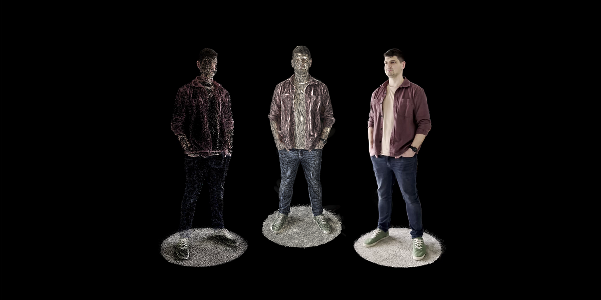
If every part seems effectively, you hopefully find yourself with a scene as proven under. Within the subsequent part we leap into the visualization and postprocessing.

You’ll be able to really see fairly good the gaussian form of particular person splats in low density areas.

Publish Processing

Although the Gaussian splatting repo comes with its personal visualizer, I choose to make use of Tremendous Splat since it’s rather more intuitive and you’ll immediately edit your scene.

So to get began, head the Tremendous Splat editor and open your ply-file, positioned underneath ./output/<RUN_NAME/point_cloud/iteration_xxxx>.

I often begin to take away many of the background factors utilizing a sphere as indicated under.